The measurement of coevolution in the wild
TLDR
Click on functions.R
for an R script that includes tools for computing and
maximizing the likelihood function of our model and for computing the
maximum likelihood values of selection strengths and optimal offset.
Tutorial
This is a tutorial for the method of coevolutionary inference introduced by Week & Nuismer (2019). Data used in this tutorial comes from Toju & Sota (2006) and have been collected here. A detailed treatment of our model, application of likelihood and analysis of data can be found in the appendix of Week & Nuismer (2019), linked to here. Aside from the derivation of equilibrium expressions, all of our calculations have been carried out in the statistical programming language R.
Introduction to the biology
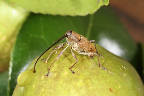
To demonstrate the utility of our method, we walk through each step taken to obtain the results produced in the main text. We restrict our analysis in this document to the data provided by Toju & Sota (2006). This paper documents the antagonistic interaction between the female Curculio camelliae weevil and the Camellia japonica fruit. Female weevils bore holes into the woody pericarps of the camellia to oviposit. Inside the fruit, weevil larvae feed on the seeds of the camellia up until the fourth instar, at which time they exit the fruit and overwinter. These two species co-occur across Japan, although camellia populations where the weevil is absent have been documented. A great deal of evidence has been produced to demonstrate that the thickness of the camellia pericarp and the length of the weevil rostrum have coevolved. In this tutorial we will be measuring the strength of coevolution and testing the hypothesis that the spatial patterns of elongation in these traits are the products of coevolution.
Phenotypic data
Estimates of mean trait pairs across multiple locations comprise the core data required to utilize this method. With these data we calculate the metapopulation mean traits, variance of local mean traits across space, and the spatial covariance of local mean traits for the two interacting species. To begin we read in the trait data to a dataframe in R. Note that although the file is named toju_pairs.Rda, we refer to it within the R environment as toju_df.
# read in data
load("measuring_coevolution_files/toju_pairs.Rda")
head(toju_df)
rostrum body pericarp location island
1 9.63 8.40 5.42 Nodzumi HNS
2 7.98 6.95 4.32 Kamo HNS
3 9.13 7.82 3.88 Nagaoka HNS
4 10.42 8.19 6.07 Kutsuki HNS
5 10.79 7.87 4.90 Hiratsuka HNS
6 9.89 7.86 6.30 Kyoto HNSNote the column names in this data frame. The column rostrum contains the mean rostrum lengths at each location used in our analysis. Column body contains the mean body sizes of weevils in each population. Column pericarp contains the mean pericarp thickness at each location. Column location contains the names of each location which we keep identical to those used in Toju & Sota 2006. Finally, the island column contains the islands for which each of these locations belong. We can visualize these data with following line of code:
# plot data
library(ggplot2)
library(ggdark)
library(gapminder)
library(ggthemes)
ggplot(toju_df, aes(x = rostrum, y = pericarp, color = island)) + geom_point() +
    dark_mode(theme_minimal()) + xlab("Rostrum length") + ylab("Pericarp thickness")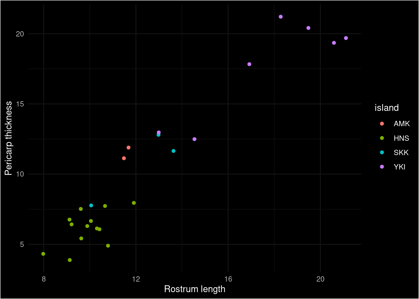
Figure 2: Displayed in this scatter plot are mean trait pairs for various locations across Japan. The colours indicate which island these locations belong to.
Background parameters
Before we can infer the strengths of biotic selection we need to infer some key background parameters. Specifically, we need to know the abiotic optima, the effective population sizes and additive genetic variances.
Abiotic optimal trait values (\(\theta_i\))
These parameters represent the trait values that maximize fitness for each species ignoring the effects of the interaction. They are potentially the most difficult to estimate depending on the biological details of the system being studied. There are many ways one can choose to estimate these values which will likely differ for each of the species involved in the interaction. For example, in the camellia-weevil system analyzed here, we found estimates of average pericarp thicknesses from populations where the weevils were found to be absent. Measuring mean trait values in populations where the interaction has not been taking place over evolutionary time-scales will likely be a popular method for inferring the abiotic optima. Another approach is to identify members of the population that do not partake in the interaction. In the case of the weevils, the males do not oviposit and hence are not involved with the arms race between the rostrum lengths of the female weevils and the thickness of the pericarps. We therefore assume the average rostrum length of the male weevils provides at least a crude estimate for the abiotic optimal trait value.
Effective population sizes (\(n_i\))
Effective population sizes are most readily estimated from population genomic data. Perhaps the most classic approach is through the equation
\[\Theta_i=4n_i\eta_i\]
where \(\Theta_i\) is the fundamental parameter from population genetics (not to be confused with \(\theta_i\) from above), \(n_i\) is the effective population size and \(\eta_i\) is the rate of mutation in species \(i\). Of course there are other methods, but the literature on this subject is far too vast to review in this short tutorial.
Using the above equation and the software package Migrate-n (Beerli 2006) Toju & Sota (2011) were able to provide estimates of effective population sizes from multiple locations across Japan. However, our method requires a single estimate of the effective population size. In the appendix of the associated manuscript, we show that, given estimates from multiple locations, the harmonic mean of these values is the correct value to use. That is, if \(n_{ij}\) is the effective population size of species \(i\) in location \(j\), then, given \(N\) locations, we would set
\[n_i=\frac{N}{\sum_j\frac{1}{n_{ij}}}.\]
Additive genetic variances (\(G_i\))
Heritabilities (in the narrow-sense) of traits are routinely estimated using parent-offspring regressions and other techniques. With an estimate of the heritability of the trait in species \(i\) (denoted by \(h_i^2\)) and an estimate of the phenotypic variance (\(\sigma_i^2\)) we can calculate an estimate of the additive genetic variance using the relation \(G_i=h_i^2\sigma_i^2\).
In Toju & Sota (2011) estimates for the heritability of pericarp thickness in the camellia fruit were calculated. We used the average of the heritabilities calculated. In addition to these values estimates of phenotypic variances were provided in Toju & Sota (2006) for multiple populations. As shown in the appendix of the associated manuscript, the arithmetic mean of additive genetic variances from multiple locations should be used as the effective additive genetic variance for our model. That is, given the additive genetic variance of species \(i\) in locations \(j=1,\dots,N\) (\(G_{ij}\)), we calculate the effective additive genetic variance as
\[G_i=\frac{1}{N}\sum_jG_{ij}.\]
Values of background parameters
We have collected the background parameters needed in the dataframe toju_par.Rda. In the R environment, this dataframe is referred to as par_df.
# read in parameters
load("measuring_coevolution_files/toju_par.Rda")
par_df
Gs thetas eff_ns species
1 0.5202037 5.911818 30769.50 C. camellia
2 5.2526697 6.248235 1789.99 C. japonicaThe column labelled Gs contains the effective additive genetic variances for each species. The column thetas contains the abiotic optimal phenotypes for each species, and the column eff_ns contains the the effective population sizes for each species. The column species denotes which species each estimate belongs to.
Estimating Selection
Inferring selection parameters and the optimal offset with our method is very brief. All the heavy lifting has already been done (see the associated manuscript for details). With the data and background parameters prepared, we simply load in the relevant function for calculating the maximum likelihood estimated of biotic and abiotic selection strengths and the optimal offset. We begin by calculating the five statistical moments that describe a bivariate normal distribution: the means (\(\mu_1,\mu_2\)), the variances (\(V_1,V_2\)) and the covariance (\(C\)). Note that we adjust the sample moment calculations for the variances and covariance. This is because the actual maximum likelihood estimates of these moments do not have the correction factor \(N-1\) in the denominator.
N <- dim(toju_df)[1]
mu1 <- mean(toju_df$rostrum)
mu2 <- mean(toju_df$pericarp)
V1 <- (N - 1) * var(toju_df$rostrum)/N
V2 <- (N - 1) * var(toju_df$pericarp)/N
C <- (N - 1) * cov(toju_df$rostrum, toju_df$pericarp)/N
Next we load in the file containing the functions needed.
# read in functions
source("measuring_coevolution_files/functions.R")
Finally we use the function ml_sol() to find our results.
n1 <- par_df$eff_ns[1]
n2 <- par_df$eff_ns[2]
th1 <- par_df$thetas[1]
th2 <- par_df$thetas[2]
G1 <- par_df$Gs[1]
G2 <- par_df$Gs[2]
ml_sol(mu1, mu2, V1, V2, C, n1, n2, th1, th2, G1, G2)
$A1
[1] 0.0002593573
$A2
[1] 8.053552e-06
$B1
[1] 0.0007168077
$B2
[1] 4.999954e-06
$k
[1] 4.51103And there we have it. The \(A_i\) is the strength of abiotic selection of species \(i\), the \(B_i\) is the strength of biotic selection on species \(i\) and the \(\kappa\) is the optimal offset. Both strengths of selection are in inverse-square phenotypic units. Since our phenotypic units are millimeters (\(mm\)), the strengths of selection found here are in \(\frac{1}{mm^2}\).
Hypothesis Testing
In this final section of our tutorial we demonstrate how to use likelihood ratios to test for the significance of coevolution. In order to solve for the above parameters, we had to maximize a function called the likelihood function. Hence, this function decreases as model parameters depart from their maximum likelihood values. In particular, when fix either \(B_1=0\) or \(B_2=0\) we obtain a restricted likelihood function, one that will never reach the actual maximum likelihood value. However, it may come very close and how close it gets will tell us something about the significance of biotic selection. In particular, setting \(L_c\) equal to the maximum likelihood value and \(L_i\) equal to the maximum possible likelihood value when \(B_i=0\), we can compute the statistic
\[\Lambda_i=2(\ln L_c-\ln L_i).\]
This is called a likelihood ratio statistic (because the difference between logs of values is equal to the log of the ratio of those values, explaining the name). This statistic is known to be approximately Chi-square distributed when sample size is sufficiently large. Since the difference between the number of parameters used to calculate \(L_c\) and the number of parameters used to calculate \(L_i\) is one (we only fix \(B_i\)), the degrees of freedom for this Chi-square distribution is one. Hence, we can use the distribution function of the Chi-square distribution to calculate the probability of observing values at least as large as \(\Lambda_i\). This probability is commonly referred to as a p-value. As we need to test both \(B_1\) and \(B_2\) for significance, we will be calculating two p-values (\(p_1\) and \(p_2\) resp). Since we are setting our significance threshold \(\alpha\) to 0.05, both \(p_1\) and \(p_2\) must be less than 0.05 for coevolution to be considered significant.
We begin by calculating the likelihoods. Since our model can capture any combination of means, variances and covariance and since the sample moments are the maximum likelihood moments, we simply plug in the sample moments to our likelihood function to obtain the maximum likelihood value. The function likelihood actually returns the log-likelihood. In the appendix we show that when \(B_1=0\) the restricted likelihood is maximized when \(\mu_2,V_1,V_2\) and \(C\) are kept at their sample moments, but \(\mu_1\) is set to \(\theta_1\). The mirror image holds for when \(B_2=0\). This is because without biotic selection there is nothing keeping the species \(i\) from evolving to its abiotic optimal value.
With these likelihoods in hand we can calculate the statistics \(\Lambda_1\) and \(\Lambda_2\). Finally, we compute the associated p-values with some built in R functions.
# preparing data for likelihood calculations
data <- cbind(toju_df$rostrum, toju_df$pericarp)
m <- c(mu1, mu2)
S <- matrix(c(V1, C, C, V2), nc = 2)

# calculating maximum likelihood
Lc <- likelihood(data, m, S)

# calculating the restricted likelihoods
L1 <- likelihood(data, c(th1, mu2), S)
L2 <- likelihood(data, c(mu1, th2), S)

# calculating the likelihood ratios
Lambda1 <- 2 * (Lc - L1)
Lambda2 <- 2 * (Lc - L2)

# calculating the p-values
p1 <- dchisq(Lambda1, 1)
p2 <- dchisq(Lambda2, 1)

# is coevolution significant?
if (max(p1, p2) > 0.05) print("Coevolution no")
if (max(p1, p2) < 0.05) print("Coevolution yes")
[1] "Coevolution yes"We see that “Coevolution yes” printed and hence coevolution was detected in this system by our method.