Stochastic Eco-Evolutionary Dynamics of Multivariate Traits
A stochastic neutral baseline for G-matrix orientation
Bob Week
KiTE Postdoc · Schulenburg Group · Kiel University
bobweek.github.io · @bweek.bsky.social
The neutral null for \(\bf G\)-matrix orientation
A standard expectation:
\[
\mathbb E[\mathbf G_t]=\mathbf G_0 e^{-t/N_e}
\]
So drift erodes heritable variation.
But because every entry shrinks proportionally,
\[
\rho\big(\mathbb E[\mathbf G_t]\big)=\rho(\mathbf G_0)
\]
Question: does the typical realized population preserve \(\mathbf G\) orientation, or only the expectation?
Drift changes individual \(\bf G\)-matrices
Classical mean behavior is correct.
But individual populations follow paths.
For nonlinear summaries such as
\[
\rho_{ij}(\mathbf G)=\frac{G_{ij}}{\sqrt{G_{ii}G_{jj}}},
\]
\[
\mathbb E[\rho(\mathbf G_t)]\neq \rho(\mathbb E[\mathbf G_t]).
\]
The puzzle
Drift is known to:
- erode heritable variation;
- generate random associations among loci;
- make replicate populations diverge.
But quantitative-genetic theory usually describes drift on \(\mathbf G\) through an expectation.
That leaves no pathwise neutral model for \(\mathbf G\) orientation.
Strategy: derive \(\bf G\) dynamics from a population process
A diffusion approximation separates robust population-level ingredients from microscopic turnover details.
Individual turnover
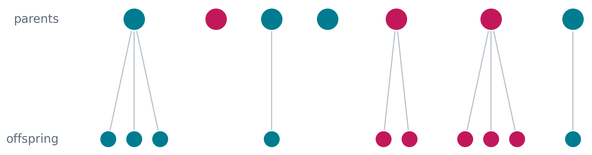
births, deaths, mutation, reproductive variance
Measure-valued diffusion
trait distribution evolves stochastically in \(\mathbb R^d\)
Moment dynamics
\(n\), \(\bar{\mathbf z}\), \(\mathbf G\), and derived quantities
Retained macroscopic ingredients:
\[
\pink{m(\nu,\mathbf z)}\quad\text{growth / selection},
\qquad
\lime{\mathbf M}\quad\text{mutation covariance},
\qquad
\violet{v}\quad\text{reproductive variance}.
\]
Heuristic picture of the diffusion limit
For one useful scaling,
\[
k\left[W^{1/k}(\mathcal P_t^{(k)},\mathbf z)-1\right]
\longrightarrow m(\nu_t,\mathbf z).
\]
Different individual-based models can share the same limit.
The point is not to keep every microscopic detail; it is to identify what survives at the population scale.
Moment equations are projections of one process
The same stochastic population process gives consistent dynamics for abundance, mean traits and covariance.
\[
\mathrm dn=\pink{\bar m n}\,\mathrm dt+\violet{\sqrt{vn}\,\mathrm dB_n}
\]
\[
\mathrm d\bar{\mathbf z}=\pink{\mathrm{Cov}(m,\mathbf z)}\,\mathrm dt
+\violet{\sqrt{\frac vn\mathbf P}\,\mathrm d\mathbf B_{\bar{\mathbf z}}}
\]
\[\begin{multline}
\mathrm d\mathbf P=\Big[\lime{\mathbf M}+\pink{\mathrm{Cov}\big(m,(\mathbf z-\bar{\mathbf z})(\mathbf z-\bar{\mathbf z})^\top\big)}\violet{-\frac vn\mathbf P}\Big]\,\mathrm dt \\
+\violet{\sqrt{\frac vn(\mathbf K-\mathbf P\otimes\mathbf P)}:\mathrm d\mathbf B_{\mathbf P}}.
\end{multline}\]
This hierarchy is not closed in general.
Gaussian closure: usable multivariate quantitative genetics
Assume additive genetic values are multivariate normal and traits decompose as
\[
\mathbf z=\mathbf g+\mathbf e,
\qquad
\mathrm{Cov}(\mathbf z)=\mathbf G+\mathbf E.
\]
Then the \(\mathbf G\) dynamics close as
\[\begin{multline}
\mathrm d\mathbf G=�igg[\lime{\mathbf M}
+\pink{2\mathbf G(\nabla_{\mathbf G}\bar m-\overline{\nabla_{\mathbf G}m})\mathbf G}
\violet{-\frac vn\mathbf G}\bigg]\,\mathrm dt \\
+\violet{\sqrt{\frac vn(\mathbf G\overline\otimes\mathbf G+
\mathbf G\underline\otimes\mathbf G)}:\mathrm d\mathbf B_{\mathbf G}}.
\end{multline}\]
This is the part I need for a stochastic neutral model of \(\mathbf G\).
Neutral \(\bf G\)-matrix dynamics under drift
\[
\mathrm d\mathbf G=
\violet{-\frac{1}{N_e}\mathbf G\,\mathrm dt}
+
\violet{\sqrt{\frac{1}{N_e}
(\mathbf G\underline\otimes\mathbf G+\mathbf G\overline\otimes\mathbf G)}:\mathrm d\mathbf B}
\]
where
\[
\frac{1}{N_e}=\frac vn,
\qquad
N_e=\frac nv.
\]
Assumptions for this neutral baseline:
- \(m(\nu,\mathbf z)\equiv0\);
- \(\mathbf M=\mathbf 0\);
- constant \(n\) and \(v\);
- no explicit recombination, selection or new mutation.
From \(\mathbf G\) to genetic correlations
Apply Itô’s formula to
\[
\rho=f(\mathbf G)=\frac{G_{ij}}{\sqrt{G_{ii}G_{jj}}}.
\]
The component form is
\[
\mathrm dG_{ij}= -\frac vnG_{ij}\,\mathrm dt
+\sqrt{\frac vn\left(G_{ii}G_{jj}+G_{ij}^2\right)}\,\mathrm dB_{G_{ij}}.
\]
The Brownian terms covary. The martingale version keeps those covariances correct while combining stochastic terms:
\[
a\,\mathrm d\mathcal M(x)+b\,\mathrm d\mathcal M(y)
=\mathrm d\mathcal M(ax+by).
\]
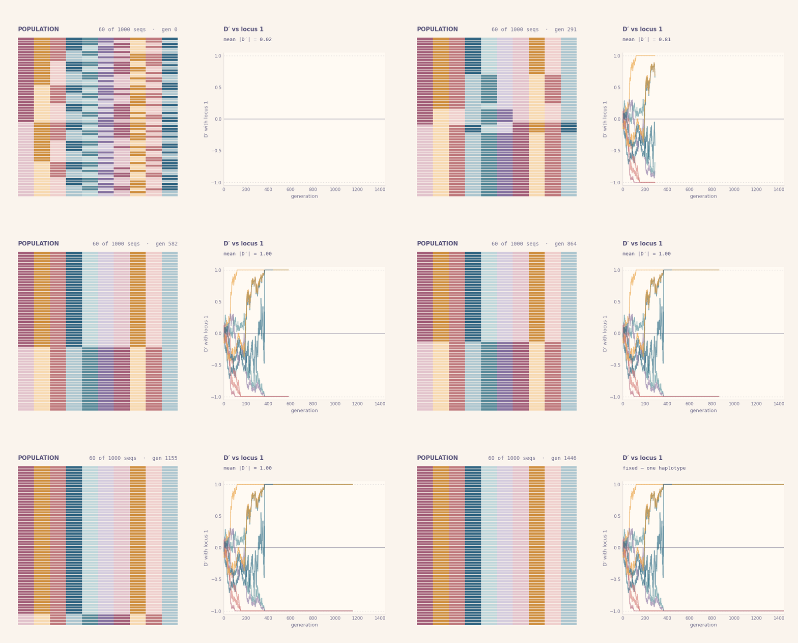
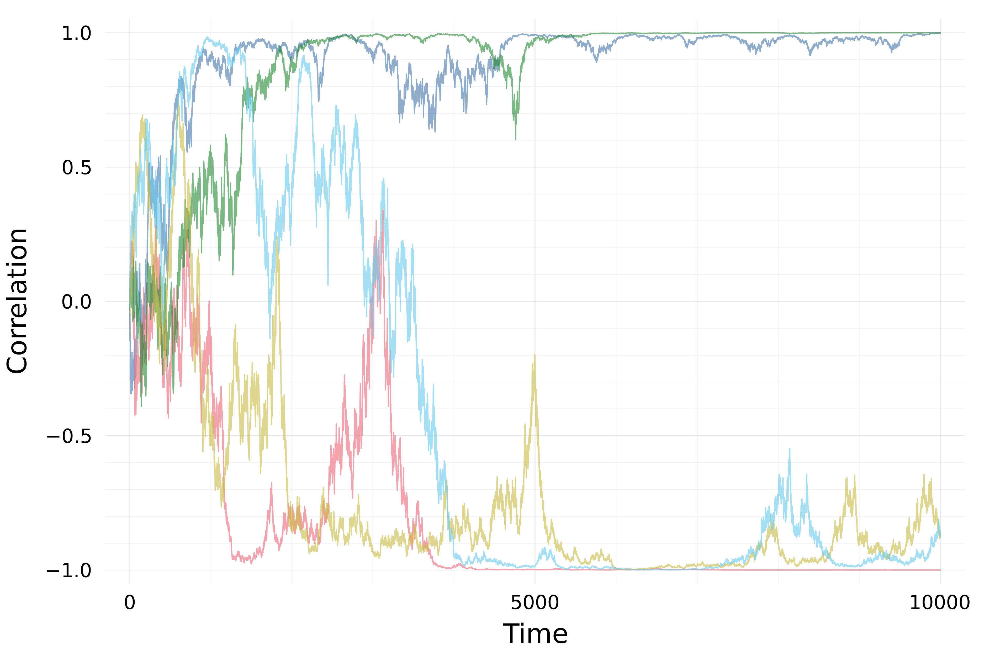
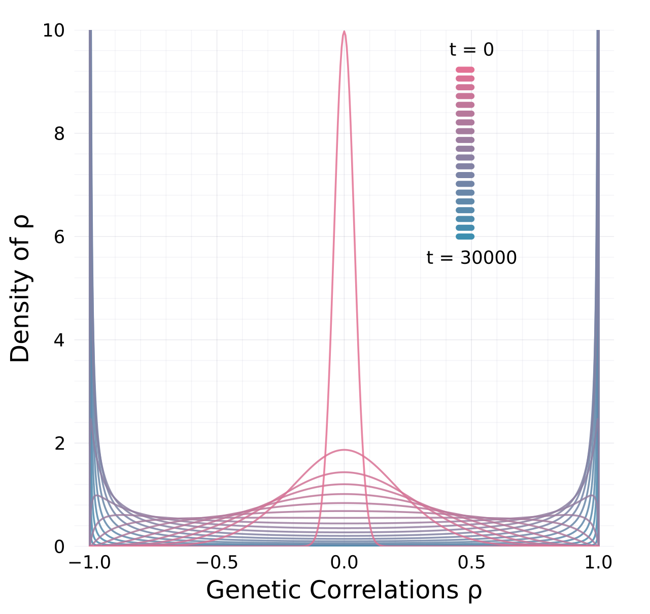
Genetic correlations tend towards \(\pm1\)
\[
\mathrm d\rho=
\pink{-\frac{1}{2N_e}\rho(1-\rho^2)}\,\mathrm dt
+
\violet{\sqrt{\frac{1}{N_e}(1-\rho^2)}\,\mathrm dB}.
\]
Under drift alone in this isolated neutral baseline, realized populations concentrate near extreme genetic correlations.
Why the drift term does not contradict this
The Itô drift term points back toward zero:
\[
-\frac{1}{2N_e}\rho(1-\rho^2).
\]
But the diffusion coefficient vanishes at the boundaries:
\[
\sqrt{\frac{1}{N_e}(1-\rho^2)}.
\]
So the process spends increasing time near \(\rho=\pm1\).
Equivalently, with \(u=\operatorname{arctanh}(\rho)\),
\[
\mathrm du = \sqrt{\frac{1}{N_e}}\,\frac{1}{\sqrt{1-\rho^2}}\,\mathrm dB,
\]
which makes boundary-seeking behavior easier to see.
Same expectation, different pathwise reality
Classical expectation:
\[
\mathbb E[\mathbf G_t]=\mathbf G_0e^{-t/N_e}
\]
Realized neutral paths:
- erode heritable variation;
- alter \(\mathbf G\) orientation;
- push genetic correlations toward extremes.
The previous null is not wrong. It is an expectation-level null, not a pathwise null for orientation.
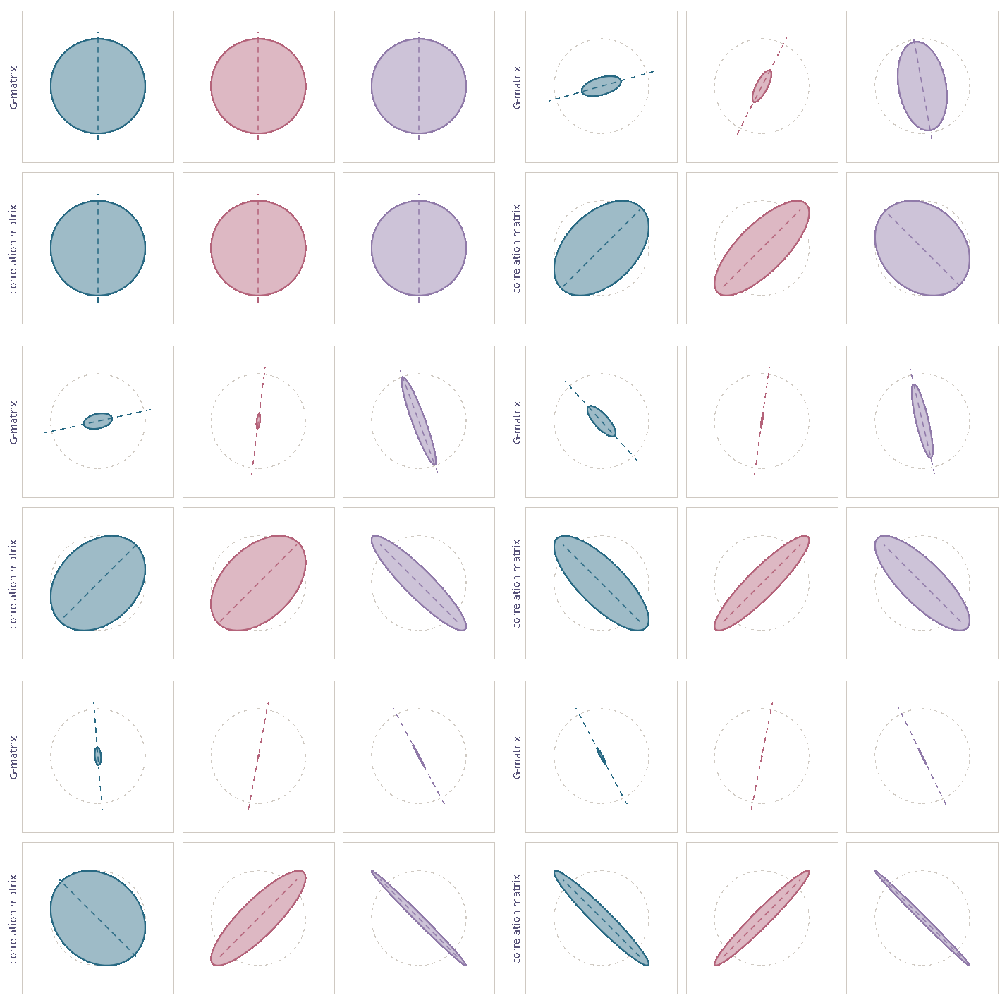
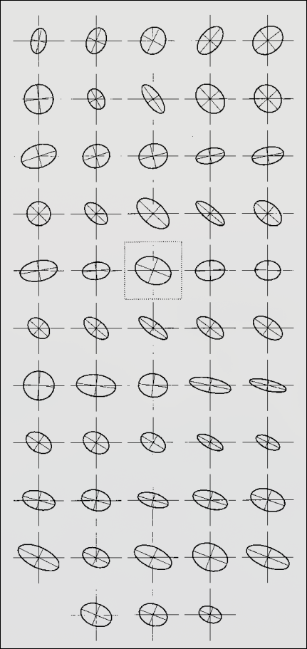
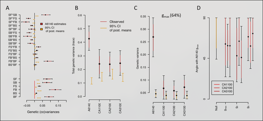
Empirical motivation: orientation can scatter under drift
Explicit recombining extensions are still needed. But these data reinforce the need for a stochastic neutral orientation baseline.
What the framework buys
Not just “moments are useful.”
The useful point is that \(n\), \(\bar{\mathbf z}\) and \(\mathbf G\) are derived from one stochastic population process, so their stochastic terms and cross-covariances are consistent.
That makes it possible to derive new stochastic dynamics for quantities such as
\[
\rho(\mathbf G),\qquad \bar m(n,\bar{\mathbf z},\mathbf G),\qquad
\alpha(\bar{\mathbf z}_1,\bar{\mathbf z}_2),
\]
rather than specifying noise terms ad hoc.
Takeaways
Drift contracts \(\mathbf G\) on average, but individual neutral paths can strongly alter orientation.
Genetic correlations tend toward \(\pm1\) in the isolated drift-only baseline.
A stochastic moment framework gives a reusable way to derive pathwise population-level models from underlying turnover.
More in the paper
![]()
Numerical implementations: github.com/bobweek/multi-mtgl
Thanks & Questions
Steve Krone, Peter L. Ralph, Hinrich Schulenburg, Patrick C. Phillips, Arne Traulsen, Jonas Wickman, Brendan Bohannan
Backup: how to choose \(m\)
The framework is useful when a biological problem can be described through growth rates or fitness functions.
Ecological examples
- Logistic growth + stabilizing selection
\[
m(\nu,\mathbf z)=r-\tfrac12\mathbf z^\top\mathbf\Psi\mathbf z-cn
\]
- Lotka–Volterra interactions
\[
m_i=r_i-\sum_j\alpha_{ij}n_j
\]
Evolutionary examples
- coevolution;
- evolutionary rescue;
- host–parasite matching;
- frequency-dependent interactions;
- density-dependent eco-evolutionary feedbacks.
Backup: analytical and numerical use
Numerical use:
- use the Brownian-motion form;
- integrate with Euler–Maruyama or SDE solvers;
- see
github.com/bobweek/multi-mtgl.
Analytical use:
- use Itô’s formula for \(\mathrm df(n,\bar{\mathbf z},\mathbf G)\);
- use martingale rules to combine correlated stochastic terms;
- avoid inventing independent noise processes where the population process says they covary.
Backup: full Gaussian closure
\[\begin{align}
\mathrm dn &= \bar m n\,\mathrm dt+\sqrt{vn}\,\mathrm dB_n,\\
\mathrm d\bar{\mathbf z} &= \mathbf G(\nabla_{\bar{\mathbf z}}\bar m-\overline{\nabla_{\bar{\mathbf z}}m})\,\mathrm dt
+\sqrt{\frac vn\mathbf G}\,\mathrm d\mathbf B_{\bar{\mathbf z}},\\
\mathrm d\mathbf G &= \left[\mathbf M+2\mathbf G(\nabla_{\mathbf G}\bar m-\overline{\nabla_{\mathbf G}m})\mathbf G-\frac vn\mathbf G\right]\mathrm dt\\
&\qquad+\sqrt{\frac vn(\mathbf G\overline\otimes\mathbf G+\mathbf G\underline\otimes\mathbf G)}:\mathrm d\mathbf B_{\mathbf G}.
\end{align}\]
Backup: reproductive variance
\(v=\) reproductive variance
Higher \(v\) means stronger demographic stochasticity and stronger random genetic drift at fixed \(n\).
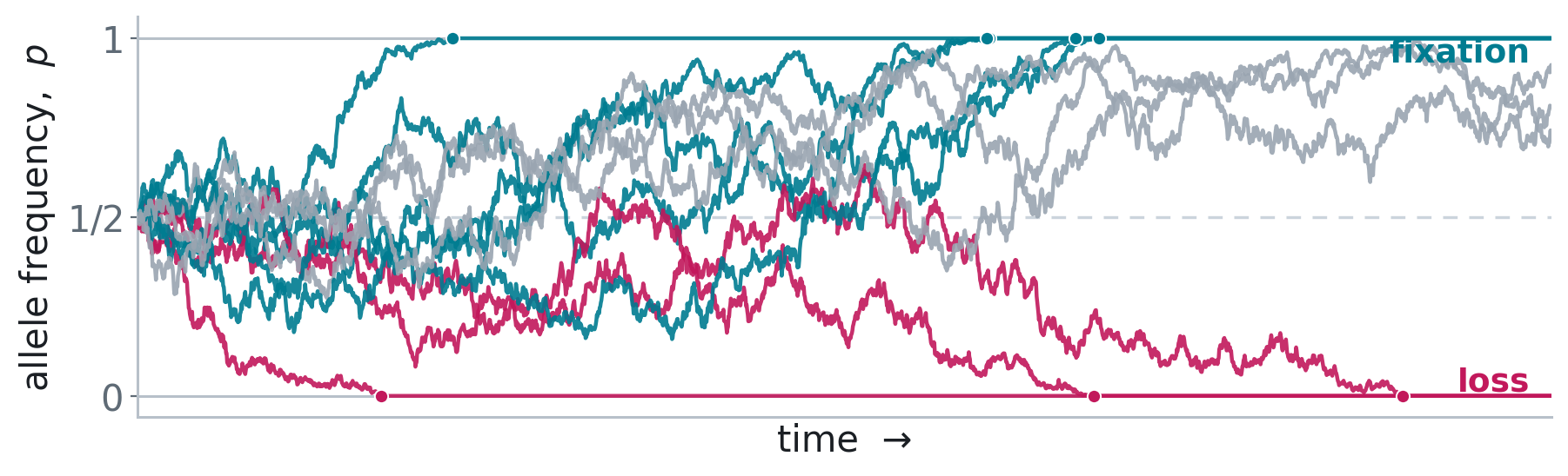
Backup: fixation intuition
\(v>0\implies\) random genetic drift