The Response of \(\bf G\)-matrices to Random Genetic Drift

and a stochastic eco-evolutionary modelling framework

Bob Week 🦠 KiTE Postdoc ~ Schulenburg Group 🪱 Kiel University

🌐 bobweek.github.io 🦋 @bweek.bsky.social

What is a \(\bf G\)-matrix?

• Multivariate trait vector: \({\bf z}=\left(\begin{smallmatrix} z_1 \\ \vdots \\ z_d \end{smallmatrix}\right)\)
• Trait decomposition: \({\bf z}={\bf g}+{\bf e}\)
  • \(\bf g=\) genetic component
  • \(\bf e=\) “environmental” component (error, everything else)
• Genetic covariance structure: \({\bf G}=\mathrm{Cov}({\bf g})=\left(\begin{smallmatrix} G_{11} & \cdots & G_{1d} \\ \vdots & \ddots & \vdots \\ G_{d1} & \cdots & G_{dd} \end{smallmatrix}\right)\)
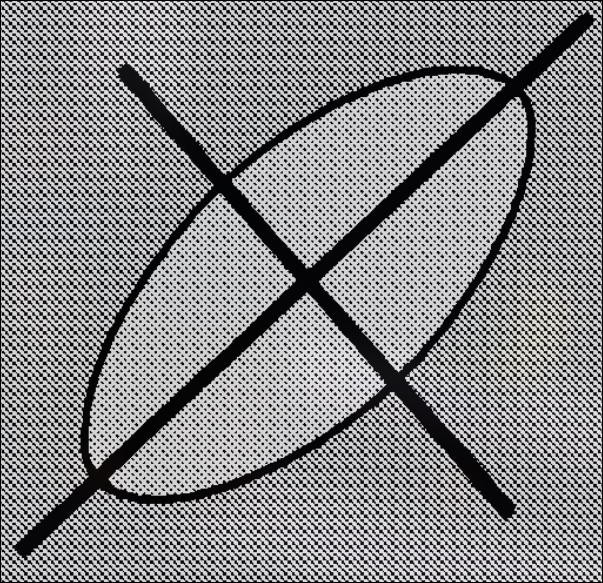
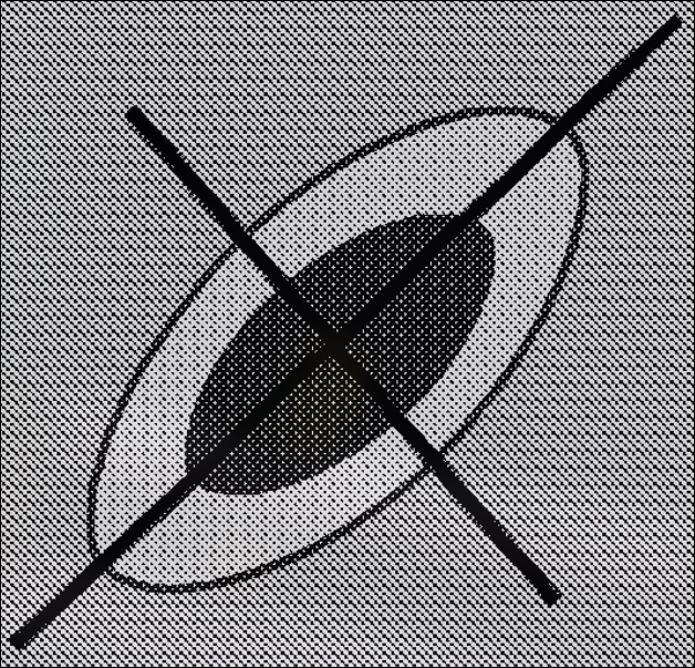
  • First two principle components:
  • Heritable component of variation
  • Predicts response to selection \(\Delta\bar{\bf z}={\bf G}\,\nabla_{\bar{\bf z}}\ln\bar W,\quad\bar W=\) mean fitness

What is random genetic drift?

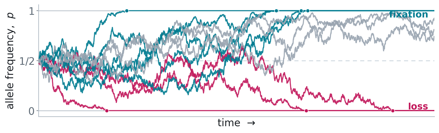
finite abundance \(\implies\) random fluctuations of allele frequencies

Response of \({\mathbb E}[{\bf G}]\) to drift

• \(\tfrac{\mathrm d}{\mathrm dt}\mathbb E[{\bf G}]\approx-\tfrac{1}{N_e}\mathbb E[{\bf G}]\), (Lande, 1979, 1980)
  
  

• \(\mathbb E[{\bf G}_t]\approx{\bf G}_0e^{-t/N_e}\)

• Drift “shrinks” entries of \(\bf G\)-matrices

The conventional view

• Drift “shrinks” entries of \(\bf G\)-matrices
• No effect on genetic correlations between traits
  • (btw, genetic correlations alter \(\bf G\)-matrix orientation)
• Differences in orientation ~ selection, mutation, migration (Roff 2000)
  
  
  • Used as evidence for selection (Cano et al. 2004)

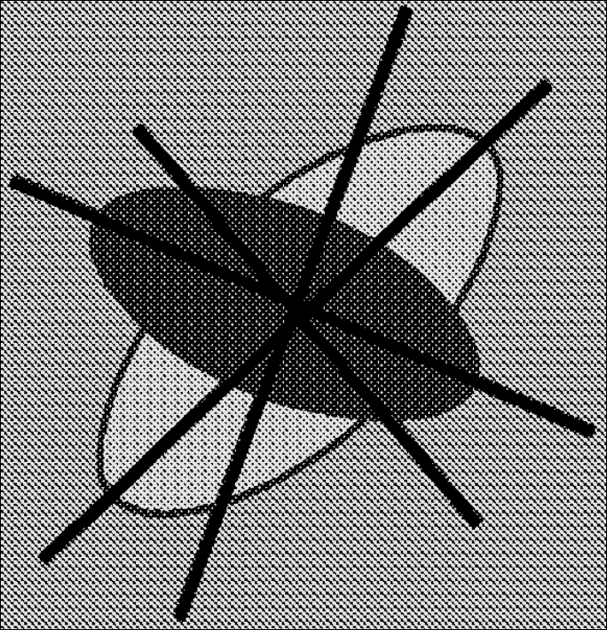
Empirical pushback and gap in theory

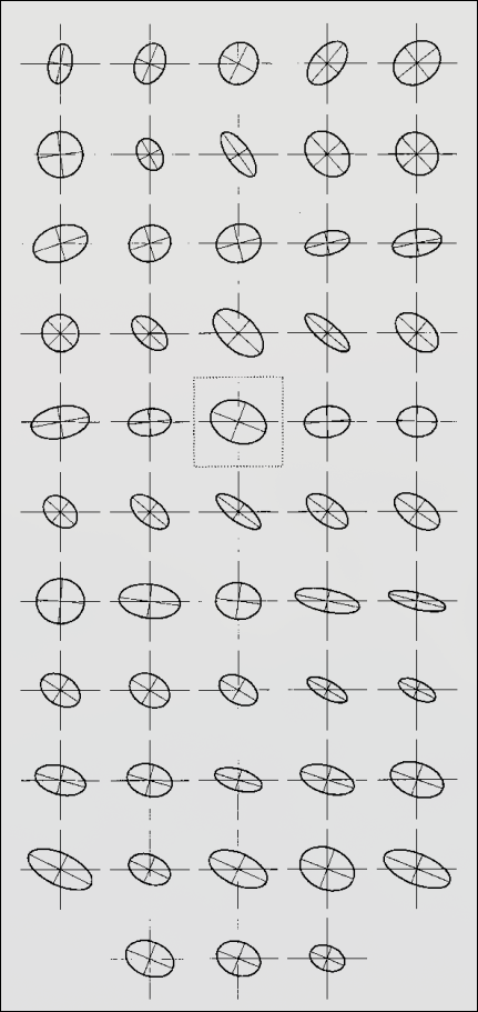
52 Drosophila lines from one ancestor: realized genetic correlations scatter across orientations and even flip sign (Phillips et al. 2001)

• Variation around \(\mathbb{E}[{\bf G}_t]\) (Phillips et al, 2001; Steppan et al, 2002)
  
  
• Still lacking stochastic neutral model (Mallard et al, 2024; Blomberg et al, 2025)

Roadmap

1. Use diffusion-limit to get SDE \(\mathrm d{\bf G}=a({\bf G})\mathrm dt+b({\bf G})\mathrm d{\bf B}\)

• Also gives abundance \(\mathrm dn\), mean trait \(\mathrm d\bar{\bf z}\)
• Also gives heuristics for calculations
  • {\(\mathrm dn,\mathrm d\bar{\bf z},\mathrm d{\bf G}\)} ∪ {heuristics} = eco-evo framework

2. Apply heuristics to study \(\mathrm d{\bf G}\)

Building the Framework

A Diffusion Approximation Approach

• Individual-Based Model:
  • Population \({\cal P}_t({\bf z})\)
  • Gaussian mutation
    • \({\bf g}'\sim{\mathrm{MVN}}_d({\bf g},{\bf M})\)
  • \(W({\cal P}_t,{\bf z})=\) fitness function

• Diffusion Limit:
  • Rescale turnover by factor \(k\)
  • Large abundance
  • Rescale population \({\cal P}_t^{(k)}({\bf z})\to \nu_t({\bf z})\)
  • Growth rate: \(m(\nu_t,{\bf z})\)
    • \(m(\nu_t,{\bf z})=\lim_k[W^{1/k}({\cal P}_t^{(k)},{\bf z})-1]k\)

Why Take a Diffusion Limit?

• Analytical tractability

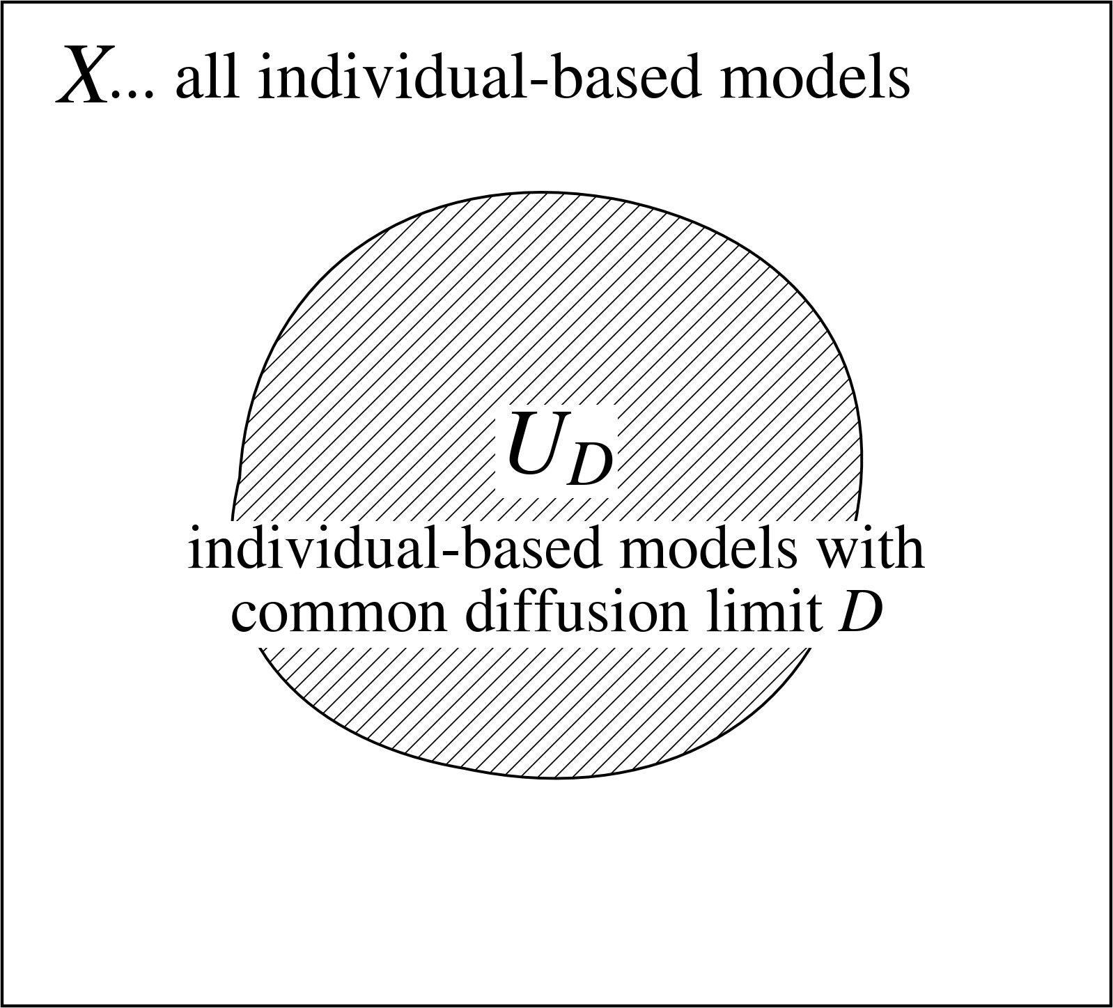
• Many models \(\rightarrow\) common diffusion limit

  • Common leading-order structure
  • Similar predictions across model class
    • (can say a lot with a little?)

• Not a universally better model

  • Depends on scaling
  • Features disappear in limit

The Diffusion Limit

Moment dynamics

● selection / growth  ● mutation  ● drift (noise)

⚠ not closed — needs \({\bf K},{\bf S},\dots\)

grows at mean fitness; demographic noise \(\propto\!\sqrt{n}\)

\[\mathrm dn={\color{#c2185b}\bar m\,n}\,\mathrm dt+{\color{#5a4cc7}\sqrt{v\,n}\,\mathrm dB_n}\]

selection moves the mean; drift jitters it

\[\mathrm d\bar{\bf z}={\color{#c2185b}\mathrm{Cov}(m,{\bf z})}\,\mathrm dt+{\color{#5a4cc7}\sqrt{\tfrac vn{\bf G}}\,\mathrm d{\bf B}_{\bar{\bf z}}}\]

mutation adds, selection reshapes, drift erodes & fluctuates

\[ \begin{aligned} \mathrm d{\bf G}=\big[&{\color{#3c8500}{\bf M}}+{\color{#c2185b}\mathrm{Cov}(m,({\bf z}-\bar{\bf z})({\bf z}-\bar{\bf z})^\top)}{\color{#5a4cc7}-\tfrac vn{\bf G}}\big]\mathrm dt\\ &+{\color{#5a4cc7}\sqrt{\tfrac vn({\bf K}-{\bf G}\otimes{\bf G})}:\mathrm d{\bf B}_{\bf G}} \end{aligned} \]

Multivariate normal approximation

ദ്ദി ˉ͈̀꒳ˉ͈́ )✧ closed

unchanged — the MVN assumption never touches abundance

\[\mathrm dn={\color{#c2185b}\bar m\,n}\,\mathrm dt+{\color{#5a4cc7}\sqrt{v\,n}\,\mathrm dB_n}\]

selection: covariance becomes a gradient of \(\bar m\) , \(\mathrm{Cov}(m,{\bf z})\to{\bf G}\nabla_{\bar{\bf z}}\bar m\)

\[\mathrm d\bar{\bf z}={\color{#c2185b}{\bf G}\big(\nabla_{\bar{\bf z}}\bar m-\overline{\nabla_{\bar{\bf z}}m}\big)}\,\mathrm dt+{\color{#5a4cc7}\sqrt{\tfrac vn{\bf G}}\,\mathrm d{\bf B}_{\bar{\bf z}}}\]

gradients again , and the noise closes: kurtosis \(\ {\bf K}\to{\bf G}\overline\otimes{\bf G}+{\bf G}\underline\otimes{\bf G}\)

\[ \begin{aligned} \mathrm d{\bf G}=\big[&{\color{#3c8500}{\bf M}}+{\color{#c2185b}2{\bf G}(\nabla_{\bf G}\bar m-\overline{\nabla_{\bf G}m}){\bf G}}{\color{#5a4cc7}-\tfrac vn{\bf G}}\big]\mathrm dt\\ &+{\color{#5a4cc7}\sqrt{\tfrac vn({\bf G}\overline\otimes{\bf G}+{\bf G}\underline\otimes{\bf G})}:\mathrm d{\bf B}_{\bf G}} \end{aligned} \]

Multivariate normal approximation

\(\partial_i:=\partial/\partial\bar z_i\) and \(\partial_{ij}:=\partial/\partial G_{ij}\).

unchanged — the MVN assumption never touches abundance

\[ \mathrm dn = {\color{#c2185b}\bar m\,n}\,\mathrm dt + {\color{#5a4cc7}\sqrt{v\,n}\,\mathrm dB_n} \]

selection covariances become gradients: \(\operatorname{Cov}(m,g_i)\to \sum_{j=1}^dG_{ij}(\partial_j\bar m-\partial_jm)\)

\[ \mathrm d\bar z_i = {\color{#c2185b} \sum_{j=1}^{d} G_{ij} \left( \partial_j\bar m-\partial_jm \right)} \,\mathrm dt + {\color{#5a4cc7} \sqrt{\frac{v}{n}G_{ii}}\, \mathrm dB_{\bar z_i}} \]

gradients again, and the noise closes: Gaussian fourth moments reduce the drift covariance to products of entries of \(\mathbf G\)

\[ \begin{aligned} \mathrm dG_{ij} ={}& \Bigg[ {\color{#3c8500}M_{ij}} + {\color{#c2185b} 2\sum_{k,l=1}^{d} G_{ik} \left( \partial_{kl}\bar m-\partial_{kl}m \right) G_{lj}} - {\color{#5a4cc7}\frac{v}{n}G_{ij}} \Bigg]\mathrm dt \\[2pt] &+ {\color{#5a4cc7} \sqrt{ \frac{v}{n} \left( G_{ii}G_{jj}+G_{ij}^{2} \right) }\, \mathrm dB_{G_{ij}}}, \qquad 1\leq i\leq j\leq d . \end{aligned} \]

How to use?

(choose \(m\) then numerical or analytical approach)

Deterministic/selection:

• \(m(\nu,{\bf z})\) very general
• Examples:
  • Logistic growth + stabilizing selection \(m(\nu,{\bf z})=r-\tfrac 1 2 {\bf z}^\top{\bf \Psi}{\bf z}-c\,n\)
  • Lotka-Volterra \(m_i=r-\sum_j\alpha_{ij}n_j\)
  • Host-Parasite Coevolution
    \(m_H({\bf z}_H,{\bf z}_P)=r+\alpha({\bf z}_H,{\bf z_P})\)
    \(m_P({\bf z}_P,{\bf z}_H)=r-\alpha({\bf z}_H,{\bf z_P})\)

Stochasticity/drift:

• No stochastic calculus needed
  • Numerical integration: github.com/bobweek/multi-mtgl
  • Analytical methods:
    • Itô’s Formula for \(\mathrm df(n,{\bar{\bf z}},{\bf G})\)
    • Heuristics for \(\mathrm d B_n,\mathrm d {\bf B}_{\bar{\bf z}},\mathrm d {\bf B}_{\bf G}\)
    • Demo with \(\mathrm d\rho\) from \(\mathrm d {\bf G}\)

The Response of \(\bf G\) to Drift

A new neutral model of \(\bf G\)-matrix evolution

\[\mathrm d{\bf G}={\color{#c2185b} -\tfrac{1}{N_e}{\bf G}\,\mathrm d t} + {\color{#5a4cc7}\sqrt{\tfrac{1}{N_e}({\bf G}\underline\otimes{\bf G}+{\bf G}\overline\otimes{\bf G})}:\mathrm d{\bf B}}\]

• \(m(\nu,{\bf z})\equiv0\)
• \({\color{#3c8500}\bf M}={\bf 0}\)
• \(N_e=n/v\) effective population size (assumed constant)
• Deterministic part ~ shrinks \(\bf G\)
  • Agrees with Lande’s \(\mathbb E[{\bf G}_t]\)
• Stochastic part ~ complicated …
  • study \(\rho_{ij}=G_{ij}/\sqrt{G_{ii}G_{jj}}\) to gain insights

Obtaining dynamics of genetic correlations \(\mathrm d\rho\)

• Use Itô’s formula on \(\rho=f({\bf G})\)

\[ \mathrm d\rho = \sum_{ij} \frac{\partial f}{\partial G_{ij}}\, \mathrm dG_{ij} + \frac{1}{2} \sum_{ijkl} \frac{\partial^2 f} {\partial G_{ij}\,\partial G_{kl}}\, \mathrm dG_{ij}\,\mathrm dG_{kl}. \]

• recall \(\mathrm dG_{ij}={\color{#c2185b}-\tfrac v n G_{ij}}\,\mathrm dt+{\color{#5a4cc7}\sqrt{G_{ij}^2-G_{ii}G_{jj}}\,\mathrm dB_{G_{ij}}}\)

  • rewrite \({\color{#5a4cc7}\sqrt{G_{ij}^2-G_{ii}G_{jj}}\,\mathrm dB_{G_{ij}}}={\color{#5a4cc7}\mathrm d{\cal M}((g_i-\bar g)(g_j-\bar g)-G_{ij})}\)

• because linearity \(a\,\mathrm d{\cal M}({x})+b\,\mathrm d{\cal M}({y})=\mathrm d{\cal M}(a\,{x}+b\,{y})\)

  • then rewrite back with \(\mathrm dB=\mathrm d{\cal M}(a\,{x}+b\,{ y})\)
  • what about \(\mathrm dG_{ij}\,\mathrm dG_{kl}\)?

Stochastic heuristics for \(\mathrm d\mathcal M(x)\)

classically: \(\mathrm dt^2=0,\mathrm dB^2=\mathrm dt,\mathrm dt\,\mathrm dB=0\)

\[x({\bf g}),\,y({\bf g}),\quad \|x\|=\sqrt{v\,n\,\overline{x^2}}, \qquad \langle x,y\rangle=v\,n\,\overline{xy} \]

scale \[ \mathrm d\mathcal M(x) = \|x\|\, \mathrm d B_{x} \] convert to Brownian noise

multiply \[ \mathrm d\mathcal M(x)\, \mathrm d\mathcal M(y) = \langle x,y\rangle\,\mathrm dt \] compute Itô terms

add \[ \mathrm d\mathcal M(ax+by) = a\,\mathrm d\mathcal M(x) + b\,\mathrm d\mathcal M(y) \] combine noise terms

Martingale-gradient version

\(\partial_i:=\partial/\partial\bar z_i\) and \(\partial_{ij}:=\partial/\partial G_{ij}\).

abundance noise is the martingale evaluated at \(1\)

\[ \mathrm dn = {\color{#c2185b}\bar m\,n}\,\mathrm dt + {\color{#5a4cc7}\mathrm d\mathcal M(1)} \]

mean trait noise tracks deviations in additive genetic values

\[ \mathrm d\bar z_i = {\color{#c2185b} \sum_{j=1}^{d} G_{ij} \left( \partial_j\bar m-\partial_jm \right)} \,\mathrm dt + {\color{#5a4cc7} \frac{1}{n}\, \mathrm d\mathcal M(g_i-\bar g_i)} \]

\(\mathbf G\) noise tracks centered products of additive genetic deviations

\[ \begin{aligned} \mathrm dG_{ij} ={}& \Bigg[ {\color{#3c8500}M_{ij}} + {\color{#c2185b} 2\sum_{k,l=1}^{d} G_{ik} \left( \partial_{kl}\bar m-\partial_{kl}m \right) G_{lj}} - {\color{#5a4cc7}\frac{v}{n}G_{ij}} \Bigg]\mathrm dt \\[2pt] &+ {\color{#5a4cc7} \frac{1}{n}\, \mathrm d\mathcal M\!\left( (g_i-\bar g_i)(g_j-\bar g_j)-G_{ij} \right)} \end{aligned} \]

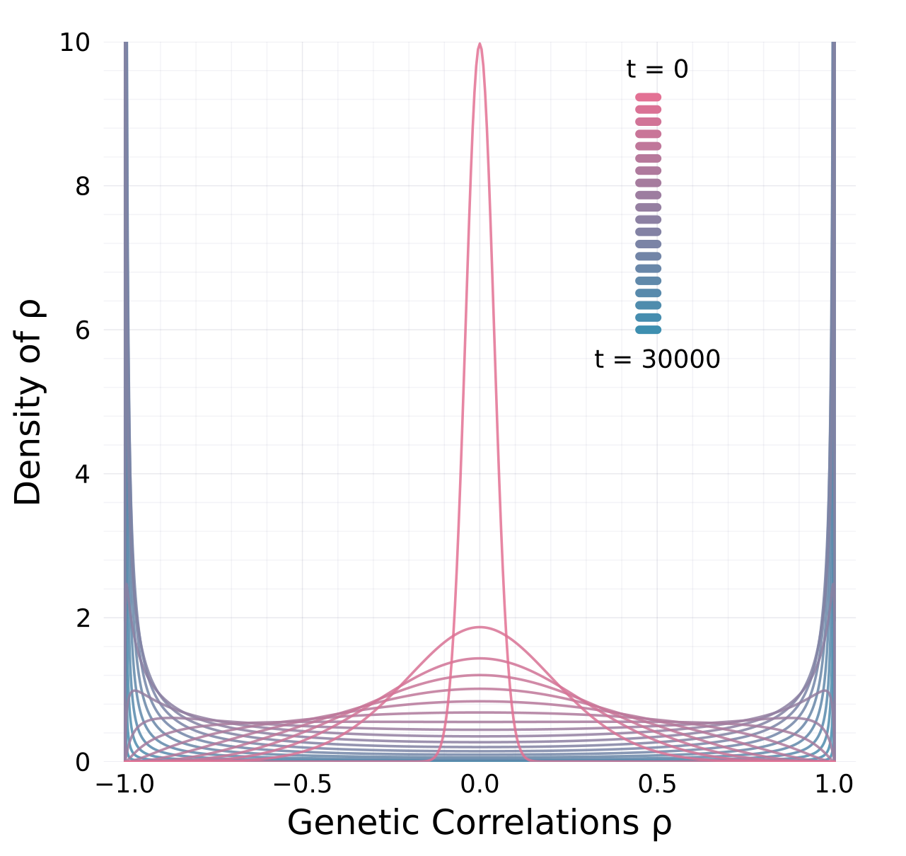
Genetic correlations tend towards ±1

\[\mathrm d\rho={\color{#c2185b}-\frac{1}{2N_e}\,\rho\,(1-\rho^2)}\,\mathrm dt+{\color{#5a4cc7}\sqrt{\frac{1}{N_e}\,(1-\rho^2)}\,\mathrm dB}\]

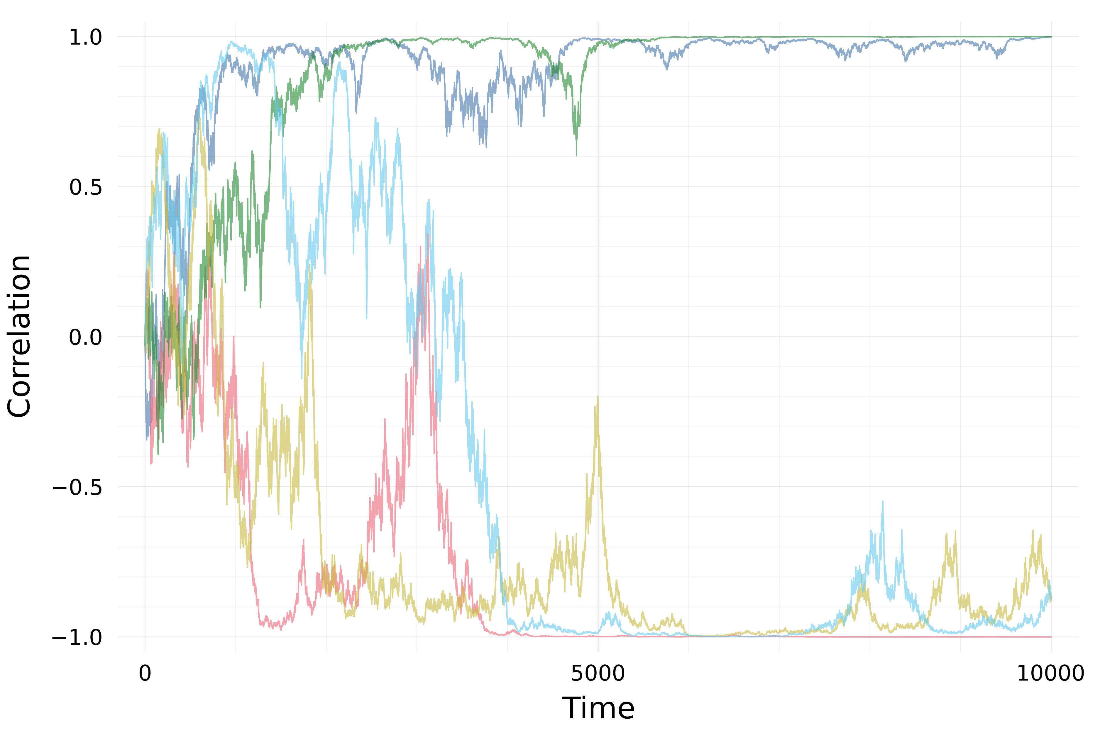
Five replicates starting at \(\rho_0=0\), with \(1/N_e=0.001\)

Evolution of pdf for \(\rho\) with \(1/N_e=0.001\)

Revised view

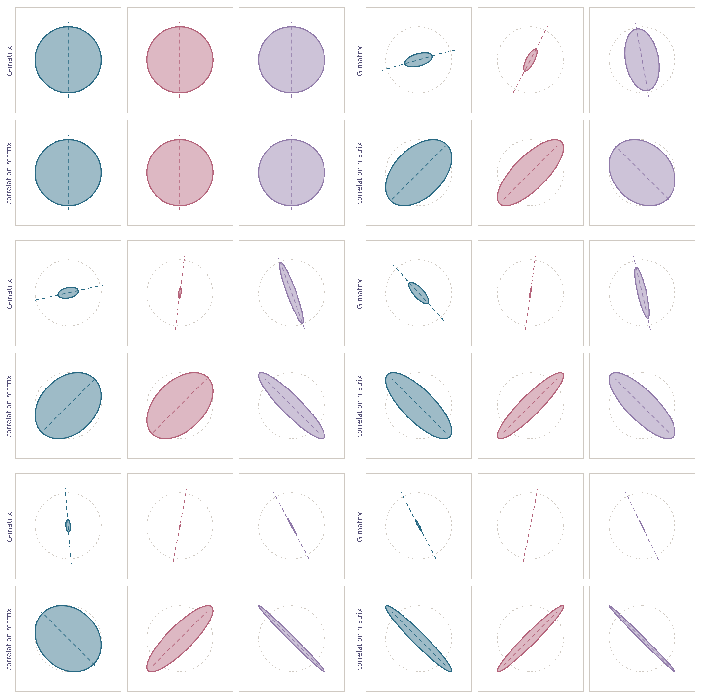
• Drift alters orientation of \(\bf G\)-matrices
  • while also eroding variation \({\mathbb E}[{\bf G}_t]\)
• Stability of \(\bf G\)-matrix structure due to
  • mutation, migration, selection
• Essentially complete opposite of previous view (Roff 2000)

More in the paper…

Conclusion

• Revised view on \(\mathrm d{\bf G}\)
• Useful set of equations and heuristics
  • increase accessibility of formal stochastic models
  • quickly obtain diverse models

Thanks & Questions

Steve Krone, Peter L. Ralph, Hinrich Schulenburg, Patrick C. Phillips, Arne Traulsen, Jonas Wickman, Brendan Bohannan

What about Recombination?

Drift alters \(\bf G\)-matrix orientation even with recombination

52 Drosophila lines from one ancestor: drift alone scatters the genetic correlation across orientations and flips its sign
(Phillips et al. 2001)

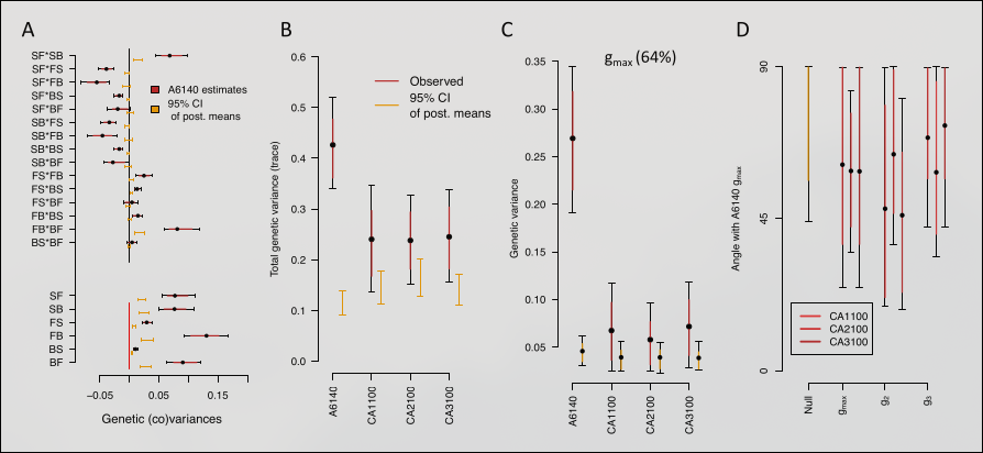
Outcrossing C. elegans, 240 generations, means static: evolved major axes randomly oriented vs the ancestor
(Mallard et al. 2023)

What about environmental stochasticity?

• \(m(\nu,{\bf z})=\) random field

• pop-gen (Gillespie 1972, 1973a, …, 1979)

• \(\mathrm d\bar{\bf z}\) (Lande 2007, 2008)

• Measure-valued (Mytnik 1996, Mytnik & Xiong 2007)